Byte-Pair Encoding for Text Tokenization in Natural Language Processing
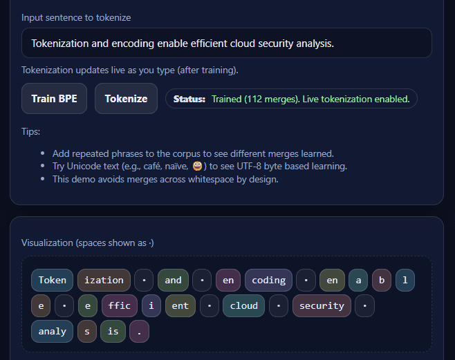
1. Introduction Modern natural language processing (NLP) systems do not operate directly on raw text. Instead, text must first be transformed into a structured representation that models can process efficiently. One of the most important steps in thi...
Feb 2, 20265 min read
![Text Representation Basics for Natural Language Processing [Interactive Simulation]](/_next/image?url=https%3A%2F%2Fcdn.hashnode.com%2Fres%2Fhashnode%2Fimage%2Fupload%2Fv1769996097089%2Fbe2ca449-7145-4a87-ae0b-c1ccd57960f2.webp&w=3840&q=75)